PaDEL-AIMA

Tutorial

1. Start MZmine using either startMZmine_Windows.bat (on Windows), startMZmine_MacOSX.command (on Mac OS X), or startMZmine_Linux.sh (on Linux/Unix systems).
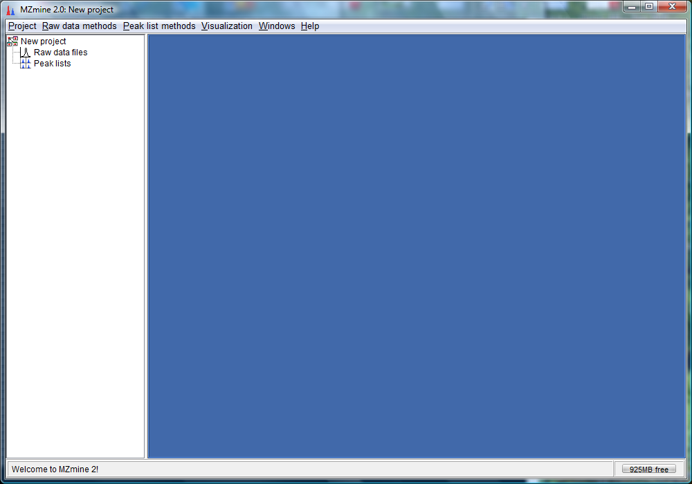
2. The start up screen for MZmine would look as follows:

   

3. Download spectra files from here. These spectra files are LC-MS subset of the data from 200-600 m/z and 2500-4500 seconds of the spinal cords of 6 wild-type(wt) and 6 FAAH knockout(ko) mice taken from Saghatelian A, Trauger SA, Want EJ, Hawkins EG, Siuzdak G, Cravatt BF: Assignment of endogenous substrates to enzymes by global metabolite profiling. Biochemistry 2004, 43(45):14332-14339.
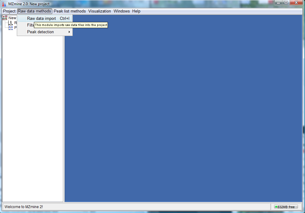
4. In MZmine, click on "Raw data methods"-->"Raw data import" as follows:

   

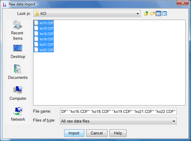
5. Select all the ko data sets as follows (to select more than one data set at a time hold on to the ctrl button while selecting) and click on import:

   

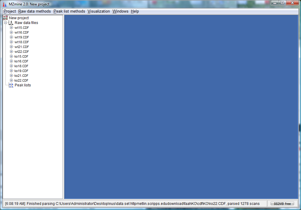
6. Do the same for the wt data sets and you would see the list of imported files as follows:

   

7. Select all the imported data sets and click on "Raw data methods"-->"Peak detection"-->"Chromatogram builder" as follows:

   

8. The following dialog box would appear:

   

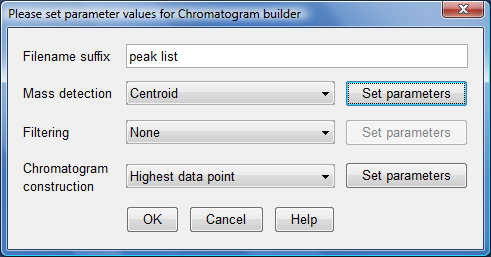
9. Click on top "Set parameter" button and another dialog box would appear:

   

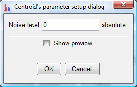
10. Ensure that the noise level is set to zero and click "OK" twice. Then you would see a Task in Progress dialog box as below. Wait until this dialog box disappears which would indicate that the processing is complete:

    

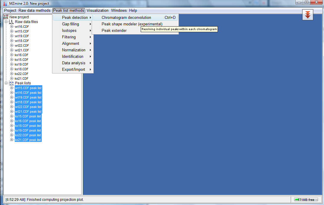
11. Now you would see new entries under Peak lists. Select all the entries under the Peak lists and click on "Peak list methods"-->"Peak detection" -->"Chromatogram deconvolution" as shown below:

    

12. This would bring up a dialog box as follows:

    

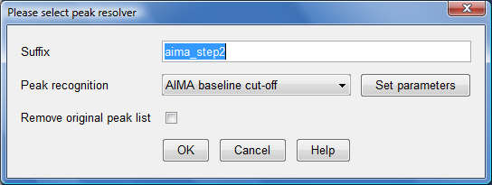
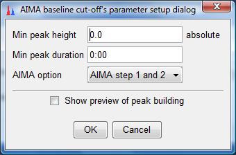
13. Click on the "Set parameters" button and another dialog box would appear. Ensure that the values are the same as indicated below and click "OK" twice. This would perform our AIMA baseline correction and create another set of entries under the Peak list.

    

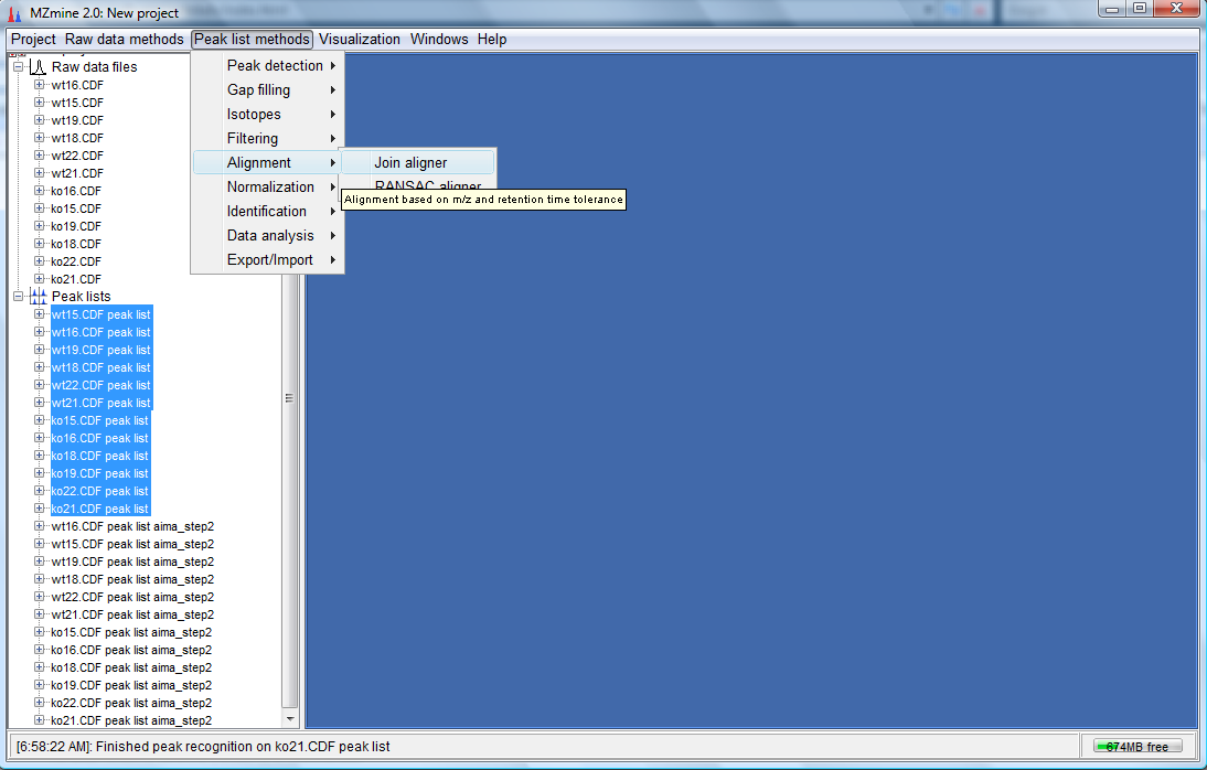
14. Before we try the PCA plot to see the difference between the peak list with and without AIMA baseline correction, we need to perform alignment. For this tutorial we would use "Join aligner". Select the peak list which was not corrected with AIMA and click on "Peak list methods"-->"Alignment"-->"Join aligner" as follows:

    

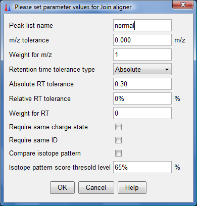
15. The following dialog would appear. Key as the parameters as shown below and click "OK".

    

16. Now do the same for the AIMA corrected peak lists by selecting them and clicking on "Peak list methods"-->"Alignment"-->"Join aligner" as shown below:

    

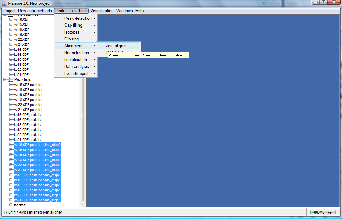
17. The following dialog would appear. Key in the parameters as shown below and click "OK".

    

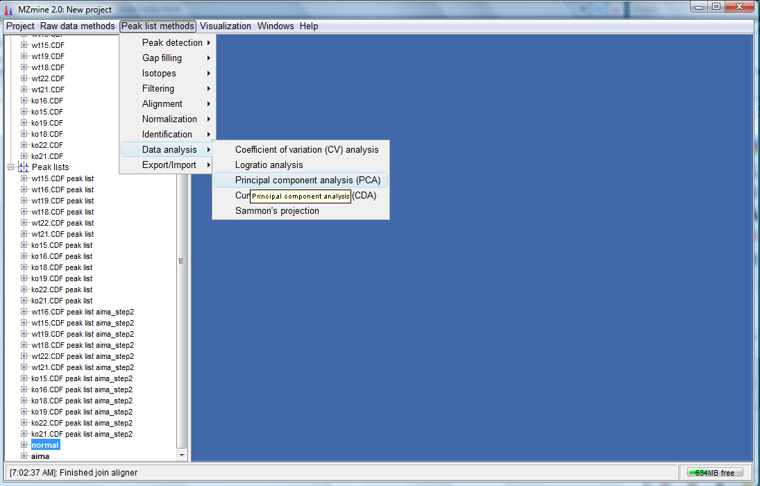
18. You would have created 2 more peak lists. One called normal and another called aima which are the aligned non-corrected and aligned AIMA corrected peak lists respectively.To perform the PCA plot, select the normal peak list and click on "Peak list methods"-->"Data analysis"--> "Principal component analysis(PCA)" as follows:

    

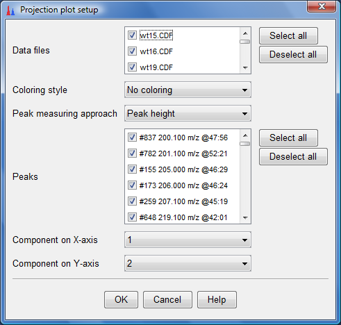
19. The dialog box shown below would appear. Click on "Select all" for both the Data files and Peaks and ensure that the other selections are as shown below. Click "OK".

    

20. To do a similar PCA plot to the AIMA corrected aligned peak list, select it and Click on "Peak list methods"-->"Data analysis"--> "Principal component analysis(PCA)" as follows:

    

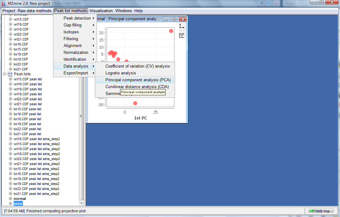
21. Click "OK" for the dialog box.
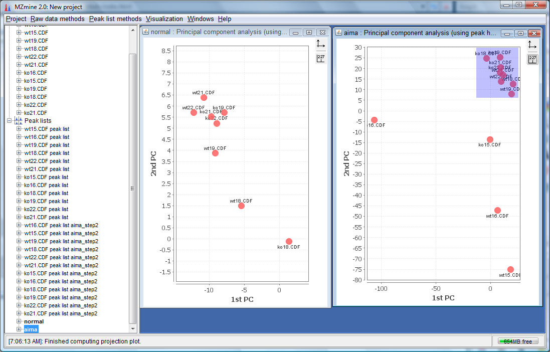
22. You would have 2 PCA plots, the non-corrected and the AIMA corrected named as "normal" and "aima" repectively as shown below:

    

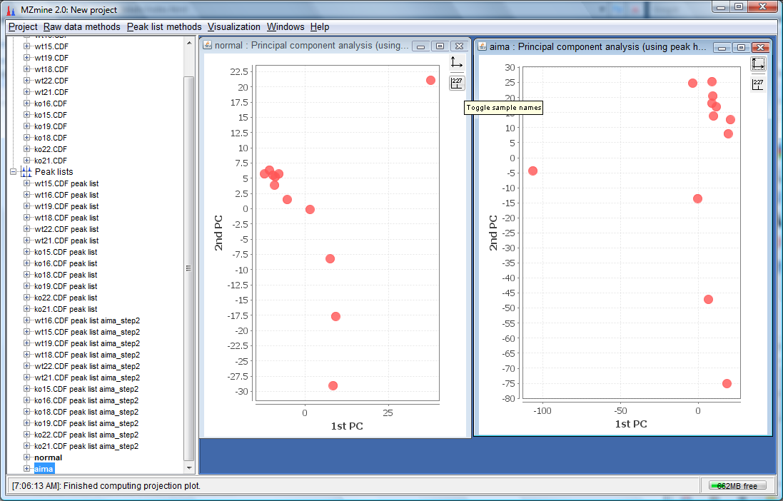
23. To see the separation improvement of AIMA more clearly, we need to zoom into the compact region for the normal plot indicated below:

    

24. For the aima corrected plot, we also need to zoom into the compact region as indicated below:

    

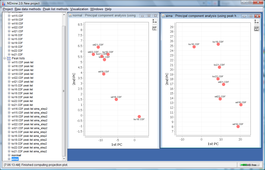
25. Finally, we can see a clearer separation of wt and ko in the AIMA corrected plot on the right as compared to normal plot on the left. The wt has moved bottom right while the ko has moved top left with a separation somewhere in the middle for the AIMA corrected plot.

    

Last modified on 3 February, 2012 by Yap Chun Wei